

Time Series Analysis
A. Introduction:
A time series is a set of numerical data obtained at regular periods of time. The statistical method used to analyze these times series data is called times series analysis. For example, if the number of students enrolled at ace Institute of Management is collected at a regular period of time then these data are referred to as time-series data since these data are collected with respect to time.
B. Components of time series:
The various factors which affect the smooth flow of time series data are termed as components of time series. The time series data are affected by the following components..
1. Long term trend or Secular trend or Trend (T)
2. Cyclic effect (C)
3. Seasonal effect (S)
4. Irregular effect (I)
1. Long term trend or Secular trend (T): The long term trend in a time series data is a general tendency of the data to increase or decrease during a long period o time. The long term trend takes the time more than one year in time series data to increase or decrease the general tendency of the data.
For example, the population has an increasing tendency during a long period of time while mortality has a decreasing tendency during a long period of time due to the advanced development in science and technology.
2. Cyclic effect (C): This cyclic effect occurred in the time series data with more than one-year period. The one complete period is called cycle. Here, data are fluctuated above and below the trend line. The time between the fluctuation of data above and below the trend
line is at least one year. The most common example of a cyclical effect is the business cycle.
3. Seasonal effect (S): Seasonal effect occurred in the time series due to the seasonal factor such as customs, religions, weather condition, tradition, culture of society etc. These seasonal factors occurred with in one year period so seasonal effects occurred in the time series data within one year period.
For example, the sale of Coca-Cola is very high during the summer seasons while the sale of coca cola is very low in the winter seasons. Hence, the data regarding the sales of coca cola is fluctuated due to summer and winter seasons.
4. Irregular variation (I): The irregular variation occurred in the time series data due to irregular factors such as earthquakes, floods, natural disasters; strikes, etc. Such types of factors are not predictable. For example, the rapid decreased in the sales of chicken meat due to bird flu.
C. Mathematical Models for Time-series:
There are two mathematical models which are adopted in the time series.
-
- Additive Model
- Multiplicative Model.
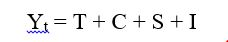
1. Additive Model: In this model, we assume that the time series data is the sum of these different components of time series i.e. long-term trend (T), Cyclic effect (C), Seasonal effect (S), and irregular effect (I).
2. Multiplicative Model: In this model, we assume that the time series data is the product of these different components of time series i.e. long term trend (T), Cyclic effect (C), Seasonal effect (S), and irregular effect (I).
![]()
D. Method of measuring the trend:
To measure the trend value, the following mathematical models are used.
- Linear Model
- Quadratic Model (Second Degree Equation)
- Linear Model: This model is same as simple linear regression model, in this model, the trend values are obtained by fitting the straight line to the given time series data set. The defined model is
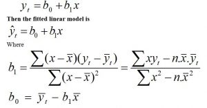
 = Trend value at a time ‘t’ or estimated value of the dependent variable.
yt = value of the variable at time‘t’.
b0 = y-intercept
b1 = slope of the trend line. This measures the average rate of increased or decreased value in the dependent variable (y) while increased the time by unit.
x = coded time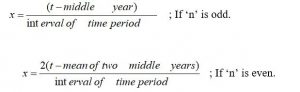
t= given time
n = number of pairs of data. - Quadratic Model (Second Degree Equation): In this model, the trend values are obtained by fitting the following second-degree equation.
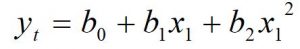
To fit this model, we need the value of b0, b1 and b2, which are obtained by solving the following three normal equations.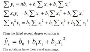 E. Short term fluctuation (Trend Eliminated Value):The difference between the observed and estimated value of the dependent variable is called short term fluctuation and it is denoted by et.
 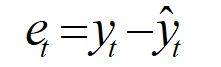 This is also known as error or residual.
F. Method of measuring the cyclical effect:
The following two methods are used to measure the cyclical effect.
i) Percent of trend
ii) Relative cyclical residual
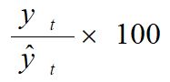
i) Percent of the trend: The measure of cyclical variation in terms of percent of trend is obtained by using the following formula.
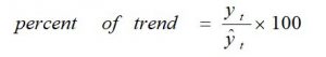
Where,
= Estimated value of the dependent variable.
yt = Value of the variable at time‘t’.ii) Relative cyclical residual: The measure of cyclical variation in terms of relative cyclical residual is obtained by using the following formula.
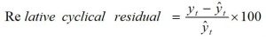
The notations have their usual meaning.G. Method of measuring the seasonal variations:
To measure the seasonal variation, we use the ration to moving average method.a. Ration to Moving Average Method Under Multiplicative Model:
The following systematic steps are used to obtain the seasonal index under this method.
Step 1– Calculate the centered 4-quarterly moving average for the quarterly data or calculate the centered 12-monthly moving average for the monthly data.
Step 2– Obtain the ratio =
 this is called ratio to moving average value which includes seasonal and irregular components of the time series.
Step 3- Make another table to calculate the seasonal indices of the following type for the quarterly data.year Trend eliminated values I Quarter II Quarter III Quarter IV Quarter –
–
–
–
–
–
–
–
–
–
Unadjusted S.I. –
–
–
–
Adjusted S.I. –
–
–
–
A similar type of table is to be formed for the monthly data.
If the sum of seasonal indices ¹ 400 for quarterly data
If the sum of seasonal indices ¹ 1200 for monthly data
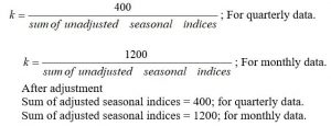
Then the seasonal indices should be adjusted by multiplying each unadjusted seasonal indices by a constant ‘k’
b. Ration to Moving Average Method Under Additive Model:
The following systematic steps are used to obtain the seasonal index under this method.
Step 1- Calculate the centered 4-quarterly moving average for the quarterly data or calculate the centered 12-montly moving average for the monthly data.
Step 2- Obtain the short term fluctuation =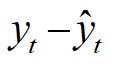
This includes the seasonal and irregular components of the time series.Step3- Make another table to calculate the seasonal indices of the following type for the quarterly data.
year Trend eliminated values I Quarter II Quarter III Quarter IV Quarter – – – – – – – – – – Unadjusted S.I. – – – – Adjusted S.I. – – – – A similar type of table is to be formed for the monthly data.
If the sum of seasonal indices ¹ 0 for quarterly data
If the sum of seasonal indices ¹ 0 for monthly data
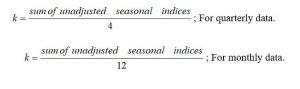
Then the seasonal indices should be adjusted by subtracting a constant ‘k’ from each unadjusted seasonal indices.
After adjustment
Sum of adjusted seasonal indices = 0; for quarterly data.
Sum of adjusted seasonal indices = 0; for monthly data.You may also like: Dummy Variables
Leave a Reply