Dummy Variables || Data Analysis and Modeling || BCIS NOTES

Dummy Variables

A qualitative (categorical) variable that can be divided into two categories by assigning 1 and 0 for the first and second category to separate these categories are called dummy variables. For example, gender is qualitative variables that can be divided into male and female categories by assigning 1 for male and 0 for female or 0 for male and 1 for female.
In dummy variables, we can not assign the number other than 0 and 1 to separate the two categories of the dummy variables. We assign the number 0 for the absence and 1 for the presence of the category.

Multiple Regression model including the Dummy Variable:
Consider the following regression model. Where x₂ is the dummy variable, represents the marital status.
X₂ = 0, for unmarried
X₂ = 1, for married.
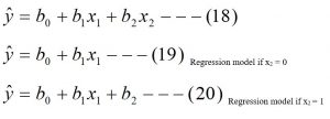
Now the model is

β0 = y-intercept.
β1 = Regression coefficient of y on x1 holding the effect of remaining variable x2 constant.
β2 = Regression coefficient of a dummy variable.
e = error term or residual.
Y = dependent variable.
X1 = independent variable.
X2 = independent dummy variable.
The fitted model is

Interpretation of regression coefficients of dummy variable:
The regression coefficient of the dummy variable measures the difference between these two categories.
If b2 = 3, this means, keeping the effect of x1 constant, in the presence of the attributed represented by 1, the value of the dependent variable is increased by 3.

If b2 = -3, this means, keeping the effect of x1 constant, in the presence of the attributed represented by 1, the value of the dependent variable is decreased by 3.

Note: the process of assigning the values 0 and 1 for the two categories is totally arbitrary but affects the sign of the value of the regression coefficient of dummy variables while interchanging the 0 and 1 values to denote these two categories. But the value to y-intercept will be changed on interchanging the 0 and 1 to denote these to categories.

Autocorrelation:
One of the basic assumptions of the regression model is that the errors are independent of one another. This assumption is often violated when data are collected over sequential periods of time because residual at any one point may tend to be similar to residual at an adjacent point in time. Such a pattern in the residual is called autocorrelation. When autocorrelation is present in a set of data, the validity of a regression model can be in serious doubt.

Residual Plots to Detect Autocorrelation:
The presence and absence of the autocorrelation can be detected by plotting residual along the vertical axis and time along the horizontal axis.
If a positive autocorrelation is present, then clusters of residuals with the same sign will be present and an apparent pattern will be readily detected.
If negative autocorrelation present, then residual will tend to jump back and forth from positive to negative to positive and so on.

The Durbin-Watson Test to Detect Autocorrelation:
The D-W test is used to detect autocorrelation. The test statistic is

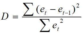
Where e_t is the residual at time ‘t’.

Decision:
For positive autocorrelation

1. If D < d_L, then errors are positively autocorrelated.
2. If D > d_u, then there is no positive autocorrelation in errors, and errors are independently distributed.
3. If d_L < D <  d_u then decision is inconclusive.

For negative autocorrelation

1. If D > 4-d_L, then errors are negatively autocorrelated
2. If D < 4-d_u, then there is no negative autocorrelation in errors, and errors are independently distributed.
3. If 4-d_u < D < 4- d_L then decision is inconclusive.

Note: When the autocorrelation is present then the least square method is not appropriate to fit the regression line. At that time we have to use other methods to fit the regression line.
Where d_L and d_u are lower and upper critical values respectively, which are obtained from the D-W table at a given level of significance and given number of independent variables.
In table ‘k’ denotes the number of independent variables and ‘n’ denotes the number of pairs of observations and µ denotes the level of significance.

Multicollinearity in Multiple Regressions:
One of the basic assumptions in a multiple regression analysis is that the explanatory variables are independent with one another but is some cases; explanatory variables are highly correlated with one another. This condition when explanatory variables are highly correlated with one another in multiple regression analysis is called Multicollinearity.

In such a situation, collinear variables do not provide new information and it becomes difficult to separate the effect of such variables on the dependent variables. In such cases, the value of the regression coefficients for the correlated variables may fluctuate drastically.

In the case of perfect Multicollinearity between the independent variables, it is not possible to estimate the separate impact of the individual independent variables on a given dependent variable.

You may also like: Analysis of Variance Table (ANOVA –Table)