Forecasting

1. Introduction:

The process of predicting the future event based on the historical (past) data is technically called forecasting. Although forecasts are critically important but they are never accurate as managers would like.

2 Evaluating the forecast accuracy:

Although forecasts are critically important they are never accurate so we have to measure the accuracy of the forecast value, whether the forecast values are either accurate or not so accurate. Mean Absolute Deviation (MAD), Mean Absolute Percentage Error (MAPE), and Mean Square Error (MSE) are used to test the accuracy of the forecast value and they are calculated by using the following relation.

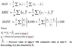
n = Number of the forecast period.
MSE = Mean Square Error
MAD = Mean Absolute Deviation
MAPE = Mean Absolute Percentage Error.

Forecasting models having a minimum value of MAD, MSE and MAPE are better than the model that has a maximum value of MAD, MSE, and MAPE i.e. how much the value of MAD, MSE, and MAPE is less; the forecast model is more accurate. The MSE is frequently used to measure the accuracy of the forecast value than others.

Note: in forecasting, the estimated value or predicted value is also denoted by Ft i.e.

Note: If the question separates the warm-up and forecasting sample, then the following points should be considered while making the forecast.

Warm-up and forecasting sample:

Before using the forecasting model to forecast future events, at first, divide the given time series data into two parts. The first part of the data is used to fit the model and this first part is called the warm-up sample. The second part of the data is used to test the accuracy of the model and this part is called the forecasting sample. There are no statistical rules to divide the data into warm-up and forecasting samples. But as far as possible, keep at least six data points or two complete seasons of seasonal data in the warm-up sample. If there are fewer data then it is not necessary to separate the time series data into warm-up and forecasting sample.

3. Forecasting models:

The following mathematical models are used to forecast the future value.

i) Naïve Model:

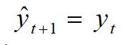
It is the simplest model of forecasting. In this model, the forecast value of any period (t+1) is the actual value of the previous period (t). The general mathematical model is

Where
= Forecast value at time (t+1).
yt = Observed data (actual data) at time‘t’
By this naïve model, we can forecast the future value only for one period ahead.

ii) Moving Average Method or Simple Moving Average Method:

In this method, we can use 2-period moving average or 3-period moving average or 4-period moving average or 5-period moving average, or any convenient period moving average method.
Here forecast value is the mean of the last n data point. For example

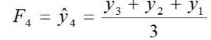
• For 3-period moving average:
The forecast value of the fourth period is the mean of the previous three-period observed values. i.e.

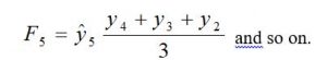
The forecast value of the fifth period is the mean of the previous three periods’ observed value. i.e.

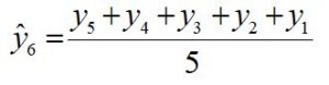
• For 5-period moving average method:
The forecast value of the sixth period is the mean of the previous five periods’ observed values. i.e.

The forecast value of the seventh period is the mean of the previous five periods’ observed values. i.e.

In a similar way, we can also use any convenient period moving average method.
By this moving average method, we can forecast the future value only for one period ahead.

iii) Trend fitting model:

This model is already discussed in the time series analysis. This model is also known as the regression model or linear model.
In forecasting, when the question mentioned about the forecasting and warm-up sample at that time, only a warm-up sample is used to fit the linear model and a forecasting sample is used to test the accuracy of the model. When the question did not mention the warm-up and forecasting sample at that time use all the data to fit the model.

iv) Simple exponential smoothing method:

In this method, the new forecast is equal to the old forecast plus a fraction of the error. The fraction (the Greek letter alpha) is called the smoothing parameter and its value lies between 0 and 1. In mathematical form, the model is

Where
= Forecast value at time (t+1).
= Forecast value at a time ‘t’ OR estimated value at a time ‘t’.
yt = observed value at time ‘t’
= Smoothing parameter and its value lie between 0 and 1.

Note: To start this method, a forecast for the first period is the mean value of the warm-up sample. Or we may take the first period’s actual value as a forecast value of the first period.

You may also like: Time Series Analysis