

Simple Regression Analysis
Regression analysis is used to measure the strength of the relationship between two or more variables. Regression analysis is used to predict or estimate the value of one dependent or response or endogenous variables based on the known values of independent or explanatory or regressor variables. The unknown variables which we have to estimate or predict are called the dependent variables and denoted by ‘y’. The variable whose value is given to estimate the value of a dependent variable (y) is called an independent variable and denoted by ‘x’.
When the regression analysis is used to measure the strength of the relationship between one dependent (y) and one independent (x) variables then it is called simple regression analysis.
1. Regression line (Regression Model)
A simple linear regression line between one dependent variable (y) and one independent variable (x1) is written as
![]()
Where
y = dependent variable
x1 = independent variable.
b0 = y-intercept for the population.
b1 = slope for the population. i.e. Regression coefficients of dependent variably (y) on independent variable (x1).
e = error term, is the difference between the observed and estimated value of the dependent variable (y)
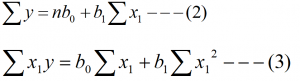
To obtain the best fit of the regression model of y on x, we need the value of b0 and b1, which are unknown. By using the principle of lest square, we can get two normal equation of regression model (1).
The two normal equation of regression line (1) are
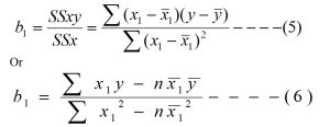
By solving these two normal equations we get the value of b0 and b1 as
![]()
After finding the value of b0 and b1, we get the required fitted regression model of y on x as
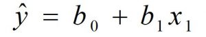
Where
![]() = estimated value of dependent variable (y) for some given value of independent variable (x1)
= estimated value of dependent variable (y) for some given value of independent variable (x1)
x1 = independent variable.
b0 = estimated value of β0 i.e. y- intercept.
b1 = estimated value of β1 i.e. regression coefficient of y on x1 or slope of the regression line.
n = Number of pairs of data.
![]() = mean of the independent variable
= mean of the independent variable
![]() = mean of the dependent variable.
= mean of the dependent variable.
3 Interpreting the regression coefficients:
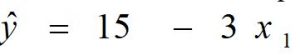
Suppose we have the fitted simple regression model
a. The coefficient ‘b0’ (estimated value of β0) represents the average value of the dependent variable (y) when value of independent variable (x1) is zero.
For example, in the above model, b0 = 15, this means, the average value of the dependent variable (y) is 15 when x1 = 0.
b. The regression coefficient ‘b1¬’ (estimated value of β1) measure the average rate of increase or decrease in the value of dependent variable (y) while increasing the value of independent variable (x1) by unit.
For example, in the above model, b1 = -3, this means, the value of dependent variable (y) is decreased by 3 while the value of independent variable (x1) is increase by 1.
Note: If in the above model b1 = 3, this means, the value of dependent variable (y) is increased by 3 while the value of independent variable (x1) is increase by 1.
4 Error term (Residual):
The difference between the observed and estimated value of the dependent variable (y) is called error or residual and it is denoted by ‘e’
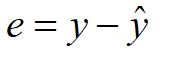
Where
e = Error term
y= Observed value of the dependent variable.
![]() = Estimated value of the dependent variable for a given value of independent variable.
= Estimated value of the dependent variable for a given value of independent variable.
5 Measures of Variation:
To examine the ability of the independent variable to predict the dependent variable (y) in the regression model, several measures of variation need to be developed. In a regression analysis, the total variation or total sum of squares (SST) is subdivide into explained variation or regression sum of squares (SSR) and unexplained variation or error sum of squares (SSE). These different measures of variation are shown in the following figure.
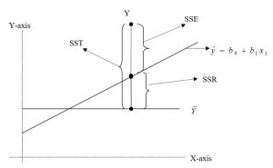
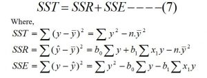
From the figure, mathematically
Total Sum of Square (SST) = Regression Sum of Square (SSR) + Error Sum of Square (SSE) i.e.
6. Standard error of the estimate (Se or Sy.x)
The standard error of the estimate measures the average variation or scatter ness of the observed data point around the regression line. Standard error of the estimate is used to measure the reliability of the regression equation and it is denoted by Se or Sy.x and is calculated by using the following relation.
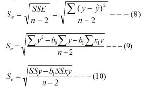
The notations have their usual meaning.
Interpreting the standard error of the estimate:
The regression line having the lesser value of the standard error of the estimate is more reliable then the regression line having the higher value of the standard error of the estimate i.e. how much the value of the standard error of the estimate is less, the fitted regression line is more reliable.
a. Is Se = 0, this means there is no variation of the observed data around the regression line i.e. all the observed data lies in the regression line. So, we expect that the regression line is perfect for predicting the dependent variable.
b. If the value of Se is large then fitted regression line is poor for predicting the dependent variable since there is greater variation of the observed data around the regression line.
c. If the value of Se is small, this means there is less variation of the observed data around the regression line. So, the regression line will be better for predicting the dependent variable.
If Se = 2.5, this means, the average variation of the observed data around the regression line is 2.5.
You may also like: Simple correlation
Leave a Reply