

Confidence Interval Estimate
A confidence interval is a type of estimate computed from the statistics of the observed data. This gives a range of values for an unknown parameter (for example, the mean). The interval has an associated confidence level that gives the probability with which the estimated interval will contain the true parameter. The confidence level is chosen by the investigator. For a given estimation in a given sample, using a higher confidence level generates a wider (i.e., less precise) confidence interval. In general terms, a confidence interval for an unknown parameter is based on sampling the distribution of a corresponding estimator.
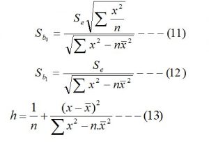
- The confidence interval for Y-intercept (β0)
![]()
2. Confidence interval for the regression coefficient or slope (β1)
![]()
3. Confidence interval estimate for the mean of the dependent variable (y)
![]()
4. Prediction interval for an individual response of dependent variable (y)
![]()
5. Approximate prediction interval: This interval gives within which the actual value of the dependent variable (Y) lies for a given value of the independent variable.
![]()
Where
![]() = Estimated value of the dependent variable for a given value of an independent variable.
= Estimated value of the dependent variable for a given value of an independent variable.
Sb0= Standard error of y-intercept (b0)
Sb1= Standard error of the regression coefficient (b1)
Se = Standard error of the estimate
tn-2, α= Tabulated value of the ‘t’ obtained from two-tailed student’s t-table at (n-2) degree of freedom and ‘µ’ level of significance.
n = Number of pairs of observations.
Other notations have their usual meanings.
Test of significance for the regression coefficient (β1):
To determine the existence of a significant linear relationship between the dependent variable (y) and independent variable (x1), a hypothesis test concerning the population slope (β1 i.e. regression coefficient) is made by setting the null and alternative hypothesis as stated below.
Null hypothesis (H0): β1 = 0 (This means there is no linear relationship between dependent and independent variables)
Alternative hypothesis (H1): β1 != 0 (This means there is a significant linear relationship between dependent and independent variable.) (Two-tailed)
If the null hypothesis is accepted then you can conclude that there is no linear relationship between dependent and independent variables. But if an alternative hypothesis is accepted then you can conclude that there is a significant linear relationship between dependent and independent variables.
Test Statistics:
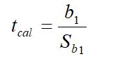
This test statistics follow t-distribution with (n-2) degree of freedom.
Decision: if the calculated value of the test statistics (tcal) is less than the tabulated value (ttab) then the null hypothesis is accepted otherwise null hypothesis is rejected. i.e.
If tcal < tµ, n-2, then the null hypothesis is accepted. Otherwise, an alternative hypothesis is accepted.
Where
tµ, n-2 = Tabulated value of ‘t’ at (n-2) degree of freedom and ‘µ’ level of significance, obtained from two tailed t-table.
n = number of pairs of data.
µ = level of significance
b1 = Regression coefficients of y on x1.
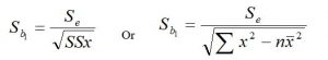
Sb1= Standard error of the regression coefficient (b1)
Other notations have their usual meanings.
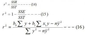
Coefficient of determination (r2):
The coefficient of determination measures the strength or extent of the association that exists between the dependent variable (y) and independent variable (x1). It measures the proportion of variation in the dependent variable (y) that is explained by the regression line. In other words, the coefficient of variation measures the total variation in the dependent variable due to the variation in the independent variable, and it is denoted by ‘r2’. The following relations are used to obtain the value of the coefficient of determination.
Note: Since the coefficient of determination is the square of the Correlation coefficient. So, the correlation coefficient is the square root of the coefficient of determination and can be obtained from the coefficient of determination by the following relation.
![]()
If the regression coefficient (b1) is negative then take the negative sign.
If the regression coefficient (b1) is positive then take the positive sign.
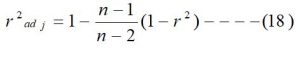
The adjusted coefficient of determination (r2adj.): The adjusted coefficient of determination is calculated by using the following relation.
Interpretation of the coefficient of determination (r2):
The regression model has a higher value of coefficient of determination is better, more reliable than the regression model having a smaller value of the coefficient of determination, this means a higher value of r2 is better than a lesser value of r2.
For example, if r2 = 0.91, this means 91% of the total variation in the dependent variable (y) is due to the variation in the independent variable (x1), and the remaining 9% variation in the dependent variable is due to the other factor which is not accounted in the independent variable.
An assumption on Regression Analysis:
The following three assumptions are necessary for the regression analysis. Which are described as,
- Normality of errors
- Homoscedasticity
- Independence of errors
- Normality of errors: This assumption requires that the errors around the regression line be normally distributed for each value of X (independent variables). As long as the distribution of the errors around the regression line for each value of independent variables is not extremely different from a normal distribution, then inference about the line of regression and regression coefficients will not be seriously affected.
- Homoscedasticity: This assumption requires that the variation around the line of regression be constant for all values of independent variables(X). This means that the errors vary the same amount when X is a low value as when X is a high value. The Homoscedasticity assumption is important for using the least square method to fit the regression line. If there are serious departures from this assumption, either data transformations or the weighted least square method can be applied.
- Independence of errors: This assumption requires that the errors around the regression line be independent for each value of explanatory variables. This is particularly important when data are collected over a period of time. In such a situation, errors for a specific time period are often correlated with those of the previous time period.
Residual analysis:
The residual analysis is a graphical method to evaluate whether the regression model that has been fitted to the data is an appropriate model. In addition, residual analysis enables potential violations of the assumption of the regression model.
The aptness of the fitted regression model is evaluated by plotting the residual on the vertical axis against the corresponding X values of the independent variable along the x-axis. If the fitted model is appropriate for the data then there will be no apparent pattern in this plot. However, if the fitted model is not appropriate then there will be a relationship between X values and the residual (e).
By plotting the histogram, box-and-whisker plot, stem-and-leaf display of the errors term, we can measure the normality of the errors.
You may also like: Simple Regression Analysis
Leave a Reply