
Demand and Supply Curve of a Firm for an Input
The market input demand curve is obtained by a lateral summation of all the individual firms’ input demand curves. This involves aggregating the demand curves of firms belonging to one industry, as well as aggregating across industries since most inputs are not industry-specific. For instance, raw cotton is used in textile as well as drug industries. Steel is used in many industries and electricity in all industries. To obtain the market demand for such general inputs, the input demand curves of firms must be aggregated across industries.
Three kinds of problems of aggregation impede the above process:
1. Industry-Wide Aggregation:
A monopoly’s input demand curve is also the industry’s input demand curve. But if the industry is perfectly competitive, its demand curve must be obtained by aggregating the individual firms’ input demand curves. The problem of aggregation arises because the individual firms’ input demand curves do not allow for their interdependence in the product market.
Each firm’s input demand curve is based on a constant product price. On the basis of the given product price, each firm demands more of input when it is cheaper, in the hope of selling more at the going product price. Since all firms do so, the supply of the product increases, pulling down the product price. This fall in the product price, in turn, inhibits the expansion of inputs demands at a lower price. Thus the final increase in input demand due to a lower price of the input is less than the sum of individual input demand curves.
Illustration – Short Run:
This can be illustrated as follows:
Suppose materials are the only variable input in the short run. Figure 13.3(a) shows the firm’s input demand curve pp x FM, at the going product price pp determined in the product market shown in Fig. 13.3(b). The changes due to a fall in the price of materials are shown by arrow marks, which are numbered in a logical sequence.
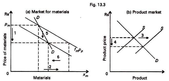
At a lower input price, the firm demands more materials as indicated by its demand curve pp x FM, in the hope of selling more at the going product price. Since all the firms do so, the product supply curve shifts to the right. This depresses the product price. At a lower product price, the input demand is less so that the firm’s input demand curve pp x FM falls. This fall reduces the expansion in demand for materials at a lower price.
DD:
The actual change in the firm’s input demand, after allowing for the changes in the product price, is shown by the demand locus DD. By summing up the demand loci DD of all the firms in the industry, we can get a competitive industry’s demand curve for an input.
The demand loci DD will have a steep slope if the change in the product price is large since pp x FM will fall by more in that case. On the other hand, a small change in the product price will yield a gently sloping DD. Whether the product price changes by much or little in the given supply conditions depends upon the elasticity of product demand. If the product demand is highly elastic, the fall in the product price will be less than if the product demand is less elastic. Thus, the elasticity of product demand affects the elasticity of input demand of the industry, in the short run.Demand and Supply Curve of a Firm for an Input
Long Run:
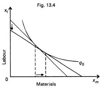
In the long run, all inputs are variable. Hence we cannot use the above apparatus for analysis. However, product price changes, in the long run, have a simple effect. They peg the size of the firm to the optimum scale of production.
Let us call the production at the optimum scale – q0. If the optimum scale of production q0 is not affected by changes in input price, a simple conclusion follows. The long-run increase in a firm’s demand for input when it becomes cheaper depends only on the elasticity of substitution at the optimum scale of production. This is illustrated in Fig. 13.4. Thus, the slope of the firm’s input demand loci DD, in the long run, depends upon the elasticity of substitution. By aggregating the individual demand loci, we get the long-run input demand curve of the competitive industry.
2. Aggregation across Industries:
When inputs are not industry-specific, their demand curves have to be aggregated across industries to get their market demand curve. Industries are vertically as well as horizontally interdependent. That is to say, the products of some industries are used by others, and products of several industries are purchased in ‘bundles’. This extensive interdependence can only be tackled in a general equilibrium framework.
It is not possible to predict a priori the results of aggregation across industries. However, we assume that the ‘law of demand’ is preserved in aggregation across industries. That is to say, the market input demand curve slopes down to the right.
3. Aggregation and Final Demand:
The price received by inputs becomes someone’s income at one stage or another. In case of payments to land, labour, capital and entrepreneurship, this is directly true. Incomes of the owners of these inputs determine their demand for consumer goods. Thus, final or product demand is affected by the prices of inputs.
Labour is a typical example of this problem. Labour accounts for a large part of consumer demand. Hence, the volume of employment and price of labour affects product demand. As a result, if the price of labour is lowered, the final demand gets depressed and the product price falls. This means that the marginal revenue product of labour also falls with its price.
Hence, the market demand curve for labour also shifts with a change in the price of labour. Due to this, the use of the simple supply-demand apparatus is not valid in the study of pricing in labour markets. Instead, a general equilibrium or a macroeconomic approach is warranted. Since both are outside the scope of this study, we will refer to this problem only in passing.
The Market Demand Curve and Input Pricing:
Usually, the problems of aggregating across industries and the interdependence of input prices and final demand are assumed away. The market input demand curves are obtained by aggregating the input demand loci DD of individual firms. The market input demand curves are then set against the supply curves of inputs and the input prices are determined. Thus, the pricing of inputs is treated only as a special case of pricing of goods and services in general.
Like product prices, input prices are conceived of as market-clearing prices which equate demand to supply. The demand for and supply of ingredient inputs is cleared by their equilibrium price. The equilibrium price of non-ingredient inputs, such as labour, clears the demand for and the supply of their services. The input demand curves that we have derived refer to the services of non-ingredient inputs, and to the physical quantities of ingredient inputs.
These are the conceptual note of Demand and Supply Curve of a Firm for an Input
You may also Like: Input Price under Different market
Leave a Reply